Finance Is Not Normal!

Article

A discussion of Normal distributions, their role in finance, and the consequences of faulty Gaussian assumptions for two fundamental models.

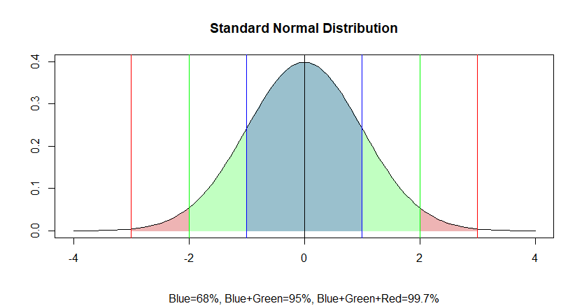
What does it mean to be normal?

When someone says a set of observations “comes from a normal distribution” most people think of a bell curve.

That is, they think of a population of observations that is centered around its mean, symmetric and for which almost all observations (99.7%) fall within three standard-deviations of the mean. The particularly astute may also note that the tail ends of the distribution contain very few observations (i.e. the kurtosis is 3). Many data sets taken from the real world are normally distributed. Consider the following distribution of heights taken from NBA players active during the 2019-2020 season.

Notice that the heights are centered around the sample mean (78.3”) and that all of the 514 observations fall between 68” and 88.7”, i.e. within three standard deviations of the sample mean. Also notice that the distribution is mostly symmetric (sample skew = 0.079) and not fat-tailed (sample kurtosis = -0.27). All in all, the normal distribution appears to be a decent fit for this data set. Due to the normal distribution’s nice mathematical properties many models, in finance and elsewhere, are built on the assumption that the underlying data is normally distributed. It is all too easy to fall into the trap of assuming that most data sets are normally distributed. When these assumptions are faulty, the consequences can be disastrous!

Where do we find Gaussian assumptions in finance?

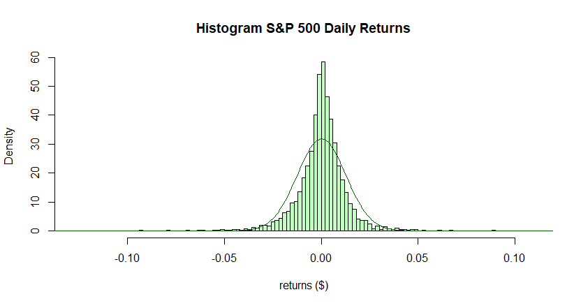
One of the most common model assumptions in finance is that an asset’s returns are log-normally distributed. Let us investigate this claim using the daily returns of the S&P 500 from January 1998 to June 2020.

The histogram above shows these returns, with a fitted normal distribution overlaid in dark green. Unlike the previous example, this dataset is not well-fit by the normal distribution. First notice that the returns are not symmetrically distributed around the mean value (0.0002), as indicated by the relatively large magnitude of the skewness (-0.3801). The tails of this distribution are also much fatter than those of the normal distribution. Only 5553/5649 (or 98.3%) of observations fall within three standard deviations of the mean (between -0.0375 and 0.0379) and the sample kurtosis is 10.43899, much higher than the kurtosis of the normal distribution. Contrary to the standard hypothesis, the S&P 500 returns do not appear to be normally distributed.

This result is not news to most people. Despite knowing this, many of the financial models used today are built on the assumption that asset returns are normally distributed. We will consider two of these models: The Black-Scholes-Merton Option Pricing Model and the Capital Asset Pricing Model.

The Black-Scholes-Merton Model

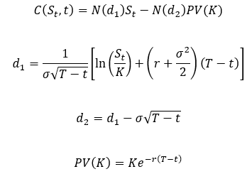
The Black-Scholes-Merton Option Pricing Model derives a formula for the value of European style options from the Black-Scholes equation. The estimated value of a call option derived from this equation is shown below.

The mathematics behind this model is somewhat complex and not the focus of this post. Instead, we should turn our attention to the use of the standard normal cumulative distribution function (specifically the and factors) in calculating the option price.

The normal cumulative distribution function appears in the pricing equation because the model is built on the assumption that the returns of the underlying asset are log-normally distributed. As we saw above, this assumption is incorrect in at least one case and has consequences for the Black-Scholes pricing model. Primarily, the predictive factors in the model ( and ) underweight the probability of tail-events occurring. Thus, the model estimate of an option’s value will likely differ from the true value.

One way we can confirm the existence of this discrepancy between the actual and Black-Scholes-predicted value of an option is by looking at implied volatility. If the Black-Scholes model were to yield accurate prices for all options contracts, then any two options with the same underlying asset and expiration date should have the same implied volatility. However, the implied volatility values for an option chain often form a “U” shape when plotted, with a much higher implied vol for deep-in-the-money and deep-out-of-the-money options than for at-the-money options.

The Capital Asset Pricing Model

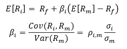
The Capital Asset Pricing Model (CAPM) relates an asset’s expected returns to systemic risk, relative to a given market.

The normality assumption comes into play when calculating β. In the above it is assumed that the entirety of the assets’ risk can be determined using only the first and second moments of the assets’ return distributions. This is only true for a select set of distributions; in this case, the assumption that a given asset’s returns follow a log-normal distribution is used to justify the calculation of β.

As we saw before, this assumption is faulty. We know that not all assets have a normal distribution’s thin tails, nor are they all symmetric about the mean, thus we need to take tail events into account when calculating risk. However, the calculation of β ignores tail dependencies between assets and thus underestimates an asset’s systemic risk, resulting in an incorrect valuation. Francois Desmoulins-Lebeault does a very thorough job exploring this phenomenon in his 2002 paper “CAPM Empirical Problems and the Distribution of Returns”.

How do we move beyond Gaussian assumptions?

We discussed how faulty normalcy assumptions can lead to inaccurate valuations for two fundamental financial models. In particular, we saw that the lack of skew and thin tails of the normal distribution can paint a false picture of an asset’s behavior.

One way to work around these issues is to use a different distribution than the normal distribution when developing financial models. One popular distribution that better captures the tail-features of the distribution of asset returns is the skewed Student’s t distribution. However, many of the common financial models are dependent on nice properties of the normal distribution, which other distributions are lacking. For this reason, using an alternative distribution is not as simple as removing a normal distribution’s fitted parameters from a model and plugging in the respective parameters from the new distribution.

The overall takeaway from this exploration is that tail events are an important aspect of financial modeling that often go understated when using Gaussian assumptions. It is for this reason that the Qdeck team pays special attention to tail events when trading. We examine benchmarks’ extreme days when evaluating a strategy and provides tools to incorporate expected tail loss when optimizing client portfolios. If one fails to account for this information when developing trading strategies, they risk significantly underestimating their true risk.

If you are curious about tools for moving beyond Gaussian distributions when dealing with multi-variate data, check out part two of this blog post: “Concerning Copula”. If you want to explore some of the Qdeck tools that target tail behavior, request a demo!

References:

“Black–Scholes Model.” Wikipedia, Wikimedia Foundation, 17 June 2020
“Capital Asset Pricing Model.” Wikipedia, Wikimedia Foundation, 1 May 2020
Desmoulins-Lebeault, François. (2003). “Distribution of Returns and the CAPM Empirical Problems.”
“Geometric Brownian Motion.” Wikipedia, Wikimedia Foundation, 27 May 2020
Kenton, Will. “Capital Asset Pricing Model (CAPM).” Investopedia, Investopedia, 30 Apr. 2020
Kenton, Will. “How the Black Scholes Price Model Works.” Investopedia, Investopedia, 2 Mar. 2020
Kenton, Will. “Understanding the Volatility Skew.” Investopedia, Investopedia, 14 Feb. 2020
Veisdal, Jorgen. “The Black-Scholes Formula, Explained.” Medium, Cantor’s Paradise, 29 Mar. 2020