By Tim Leung, Ph.D.
Market observations and empirical studies have shown that asset prices are often driven by multiscale factors, ranging from long-term economic cycles to rapid fluctuations in the short term. This suggests that financial time series are potentially embedded with different timescales.
On the other hand, nonstationary and behaviors and nonlinear dynamics are often observed in financial time series. These characteristics can hardly be captured by linear models and call for an adaptive and nonlinear approach for analysis. For decades, methods based on short-time Fourier transform have been developed and applied to nonstationary time series, but there are still challenges in capturing nonlinear dynamics, and the often prescribed assumptions make the methods not fully adaptive. This gives rise to the need for an adaptive and nonlinear approach for analysis.
Hilbert-Huang Transform (HHT)
One alternative approach in adaptive time series analysis is the Hilbert-Huang transform (HHT). The HHT method can decompose any time series into oscillating components with nonstationary amplitudes and frequencies using empirical mode decomposition (EMD). This fully adaptive method provides a multiscale decomposition for the original time series, which gives richer information about the time series. The instantaneous frequency and instantaneous amplitude of each component are later extracted using the Hilbert transform. The decomposition onto different timescales also and allows for reconstruction up to different resolutions, providing a smoothing and filtering tool that is ideal for noisy financial time series.
EMD is the first step of our multistage procedure. For any given time series x(t) observed over a period of time [0,T], we decompose it in an iterative way into a finite sequence of oscillating components cⱼ(t), for j=1, …, n, plus a nonoscillatory trend called the residue term:

To ensure that each cⱼ(t) has the proper oscillatory properties, the concept of IMF is applied. The IMFs are real functions in time that admit well-behaved and physically meaningful Hilbert transform. Specifically, each IMF is defined by the following two criteria:
- No local oscillation: the number of extrema and the number of zero crossings must be equal or at most differ by one.
- Symmetric: the maxima of the function defined by the upper envelope and the minima defined by the lower envelope must sum up to zero at any time t ∈ [0,T].
In addition, we apply the method of complementary ensemble empirical mode decomposition (CEEMD) to nonstationary financial time series. This noise-assisted approach decomposes any time series into a number of intrinsic mode functions, along with the corresponding instantaneous amplitudes and instantaneous frequencies.
Below we illustrate the intrinsic mode functions (IMFs) and residual terms from the decomposition for the S&P500 and VIX.
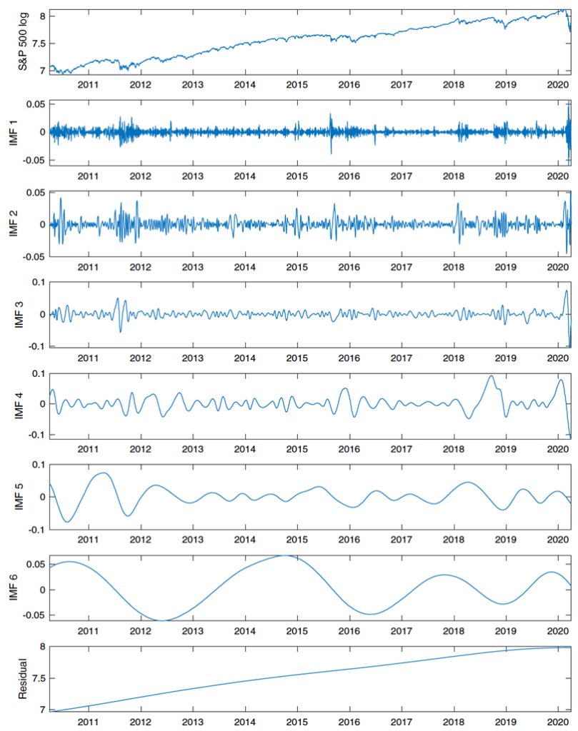
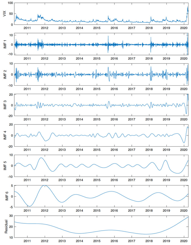
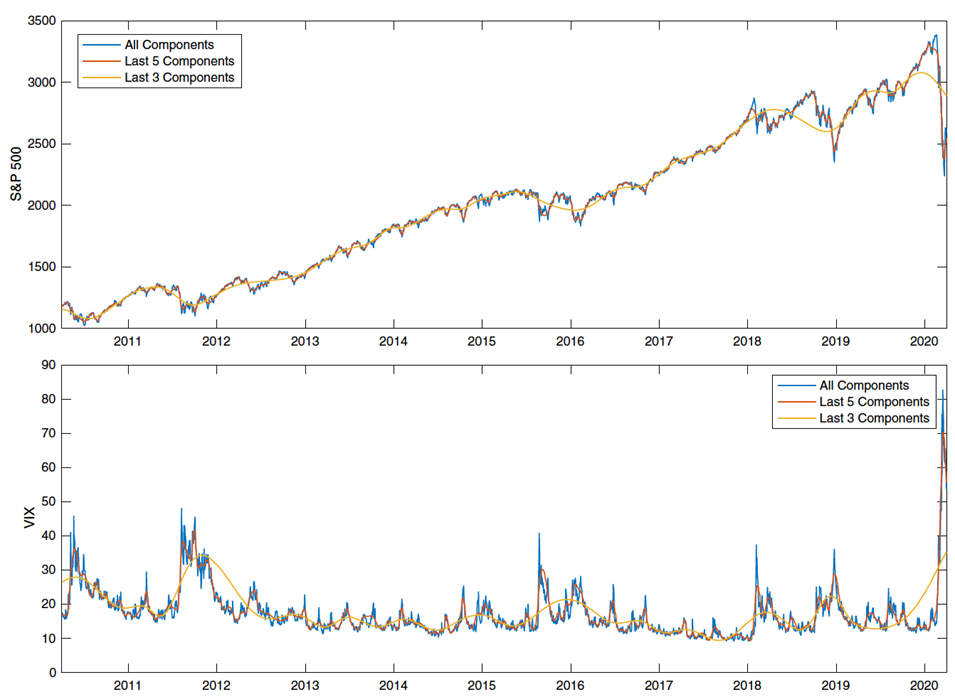
The modes correspond to different frequencies, from rapid fluctuations to long-term trends. The decomposition allows us to i) smooth/filter any time series by excluding some higher-frequency components, and ii) reconstruct any time series using a subset set of components.
Energy-Frequency Spectrum
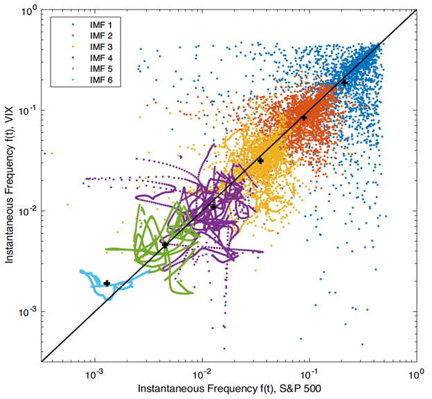
Note that each mode (IMF) also corresponds to a different frequency of fluctuations. The above decomposition allows us to compare any two time series on a mode-by-mode (frequency-by-frequency) basis.
An oscillating real-valued function can be viewed as the projection of an orbit on the complex plane onto the real axis. For any function in time X(t), the Hilbert transform is given by
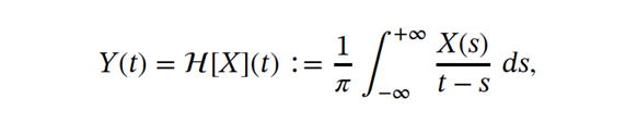
so Y(t) provides the complementary imaginary part of X(t) to form an analytic function in the upper half-plane defined by

where


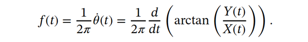
Then, the instantaneous frequency is defined as the 2𝜋 -standardized rate of change of the phase function, that is,
Applying Hilbert transform to each of the IMF components individually yields a sequence of analytic signals
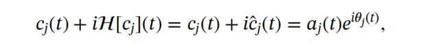
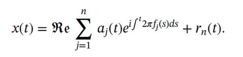
In turn, the original time series can be represented as a sparse spectral representation of the time series with time-varying amplitude and frequency:
In addition, the instantaneous energy of the jth component is defined as

Hence, for each time series, we obtain a diagram for the energy-frequency spectrum.
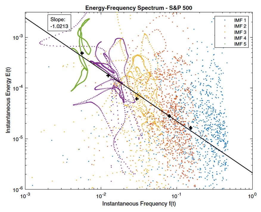
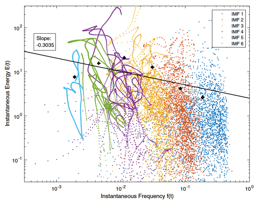
S&P500 and VIX share similar instantaneous frequencies but significantly different instantaneous energies.
In summary, the key outputs of this method are the series of IMFs, along with the time-varying instantaneous amplitudes and instantaneous frequencies. Different combinations of modes allow us to reconstruct the time series using components of different timescales. Using Hilbert spectral analysis, we compute the associated instantaneous energy-frequency spectrum to illustrate the properties of various timescales embedded in the original time series.
Multiscale signal processing is also very suitable for analyzing cryptocurrency prices (see this paper). For additional examples, such as gold (GLD) and Treasuries, along with machine learning applications, we refer the reader to the full paper.
References
Leung and Zhao (2021), Financial Time Series Analysis and Forecasting with HHT Feature Generation and Machine Learning [pdf], Applied Stochastic Models in Business and Industry
Leung and Zhao (2021), Adaptive Complementary Ensemble EMD and Energy-Frequency Spectra of Cryptocurrency Prices [pdf]
Disclaimer
This article represents the opinions and view of the author(s) and not, necessarily, of Rotella/Qdeck. The content of this article is provided solely for informational purposes and general education, and in no way should be considered investment advice.
This communication is provided for informational purposes and should not be construed as a recommendation or solicitation or offer to buy or sell futures contracts, securities or related financial instruments, nor as an official confirmation of performance. Past performance is not necessarily indicative of future results. Investment in any program is speculative and involves significant risks, including risks of loss. There can be no assurance that the programs will be able to realize their objectives.
